Penguins

Classifying Palmer Penguins with Sklearn.
Author

Trong Le

Published

March 7, 2023

In this blog post, we will use the LogisticRegression module from scikit-learn to confidently determine the species of a penguin in the smallest number of measurements necessary. Our set of data is given in the table below.

import pandas as pd

train_url = "https://raw.githubusercontent.com/middlebury-csci-0451/CSCI-0451/main/data/palmer-penguins/train.csv"
train = pd.read_csv(train_url)

from sklearn.preprocessing import LabelEncoder
le = LabelEncoder()
le.fit(train["Species"])

species = [s.split()[0] for s in le.classes_]

def prepare_data(df):
  df = df.drop(["studyName", "Sample Number", "Individual ID", "Date Egg", "Comments", "Region"], axis = 1)
  df = df[df["Sex"] != "."]
  df = df.dropna()
  y = le.transform(df["Species"])
  df = df.drop(["Species"], axis = 1)
  df = pd.get_dummies(df)
  return df, y

X_train, y_train = prepare_data(train)
X_train
Culmen Length (mm) Culmen Depth (mm) Flipper Length (mm) Body Mass (g) Delta 15 N (o/oo) Delta 13 C (o/oo) Island_Biscoe Island_Dream Island_Torgersen Stage_Adult, 1 Egg Stage Clutch Completion_No Clutch Completion_Yes Sex_FEMALE Sex_MALE
1 45.1 14.5 215.0 5000.0 7.63220 -25.46569 1 0 0 1 0 1 1 0
2 41.4 18.5 202.0 3875.0 9.59462 -25.42621 0 0 1 1 0 1 0 1
3 39.0 18.7 185.0 3650.0 9.22033 -26.03442 0 1 0 1 0 1 0 1
4 50.6 19.4 193.0 3800.0 9.28153 -24.97134 0 1 0 1 1 0 0 1
5 33.1 16.1 178.0 2900.0 9.04218 -26.15775 0 1 0 1 0 1 1 0
... ... ... ... ... ... ... ... ... ... ... ... ... ... ...
269 41.1 17.5 190.0 3900.0 8.94365 -26.06943 0 1 0 1 0 1 0 1
270 45.4 14.6 211.0 4800.0 8.24515 -25.46782 1 0 0 1 0 1 1 0
271 36.2 17.2 187.0 3150.0 9.04296 -26.19444 0 0 1 1 1 0 1 0
272 50.0 15.9 224.0 5350.0 8.20042 -26.39677 1 0 0 1 0 1 0 1
273 48.2 14.3 210.0 4600.0 7.68870 -25.50811 1 0 0 1 0 1 1 0

256 rows × 14 columns

We need to find the combination of features with which we can determine the species of a penguin the fastest. We can accomplish this by running an exhaustive search of all the features contained in this data set. At each iteration, we use the LogisticRegression module to test the score on the current set of features.

from itertools import combinations
from sklearn.linear_model import LogisticRegression

# these are not actually all the columns: you'll 
# need to add any of the other ones you want to search for
all_qual_cols = ["Clutch Completion", "Sex", 'Island']
all_quant_cols = ['Culmen Length (mm)', 'Culmen Depth (mm)', 'Flipper Length (mm)', 'Body Mass (g)']
best_score = 0
best_col = 0
for qual in all_qual_cols: 
  qual_cols = [col for col in X_train.columns if qual in col ]
  for pair in combinations(all_quant_cols, 2):
    cols = list(pair) + qual_cols
    LR = LogisticRegression()
    LR.fit(X_train[cols], y_train)
    if best_score < LR.score(X_train[cols], y_train):
        best_col = cols
        best_score = LR.score(X_train[cols], y_train)
print(best_col)
['Culmen Length (mm)', 'Culmen Depth (mm)', 'Island_Biscoe', 'Island_Dream', 'Island_Torgersen']

We can visualize the training data by using Seaborn and apply it on the most efficient combination of features that we have just found.

import seaborn as sns

# Apply the default theme
sns.set_theme()

# Create a visualization
sns.relplot(
    data=train,
    x="Culmen Length (mm)", y="Culmen Depth (mm)", col="Island", hue ='Species')
<seaborn.axisgrid.FacetGrid at 0x1f4f9fce4c0>

We can see that the training data is linearly separable. This means that the score on our logistic regression should be 100%.

LR = LogisticRegression()
LR.fit(X_train[best_col], y_train)
LR.score(X_train[best_col], y_train)
1.0

And it is 100%! Next we will try to make some interesting tables from this. First, we will divide the data set by island.

train.groupby('Island')[['Culmen Length (mm)', 'Culmen Depth (mm)']].aggregate(min).round(2)
Culmen Length (mm) Culmen Depth (mm)
Island
Biscoe 34.5 13.1
Dream 32.1 15.5
Torgersen 33.5 16.6
train.groupby('Island')[['Culmen Length (mm)', 'Culmen Depth (mm)']].aggregate(max).round(2)
Culmen Length (mm) Culmen Depth (mm)
Island
Biscoe 59.6 21.1
Dream 55.8 21.2
Torgersen 46.0 21.5

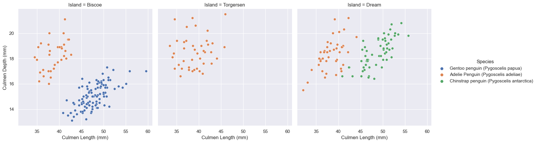
These tables give the range of culmen length and depth of the penguins on each island. For example, on Biscoe island, the culmen length range is 34.5 mm - 59.6 mm. This means that this island must have Adelie penguins on it because Adelie penguins have the shortest culmens. The 59.6 mm maximum suggests that the other species may be Gentoo or Chinstrap. The tight length range 33.5 mm - 46.0 mm suggests that there are only Adelie penguins on Torgensen island. By making quantitative comparisons like this, we can linearly separate our data.
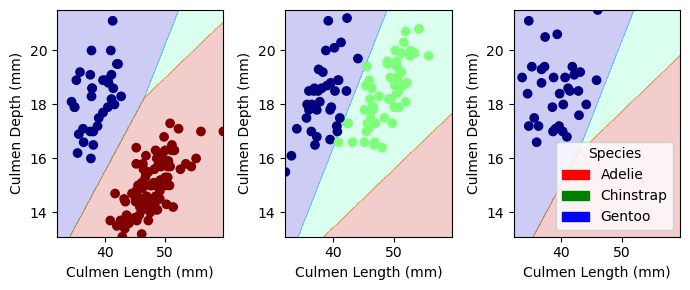
from matplotlib.patches import Patch
import matplotlib.pyplot as plt
import numpy as np

def plot_regions(model, X, y):
    
    x0 = X[X.columns[0]]
    x1 = X[X.columns[1]]
    qual_features = X.columns[2:]
    
    fig, axarr = plt.subplots(1, len(qual_features), figsize = (7, 3))

    # create a grid
    grid_x = np.linspace(x0.min(),x0.max(),501)
    grid_y = np.linspace(x1.min(),x1.max(),501)
    xx, yy = np.meshgrid(grid_x, grid_y)
    
    
    XX = xx.ravel()
    YY = yy.ravel()

    for i in range(len(qual_features)):
      XY = pd.DataFrame({
          X.columns[0] : XX,
          X.columns[1] : YY
      })

      for j in qual_features:
        XY[j] = 0

      XY[qual_features[i]] = 1

      p = model.predict(XY)
      p = p.reshape(xx.shape)
      
      
      # use contour plot to visualize the predictions
      axarr[i].contourf(xx, yy, p, cmap = "jet", alpha = 0.2, vmin = 0, vmax = 2)
      
      ix = X[qual_features[i]] == 1
      # plot the data
      axarr[i].scatter(x0[ix], x1[ix], c = y[ix], cmap = "jet", vmin = 0, vmax = 2)
      
      axarr[i].set(xlabel = X.columns[0], 
            ylabel  = X.columns[1])
      
      patches = []
      for color, spec in zip(["red", "green", "blue"], ["Adelie", "Chinstrap", "Gentoo"]):
        patches.append(Patch(color = color, label = spec))

      plt.legend(title = "Species", handles = patches, loc = "best")
      
      plt.tight_layout()
plot_regions(LR, X_train[best_col], y_train)

These 3 graphs correspond to the 3 islands: Biscoe, Dream and Torgensen.

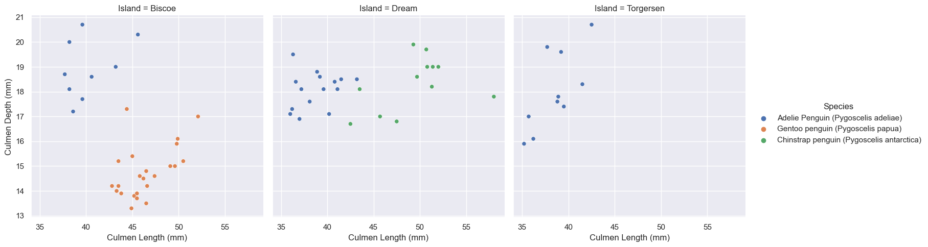
Now that we have established that “Culmen Length”, “Culmen Depth” and “Island” make the best feature combination, we will test this out on new data.

test_url = "https://raw.githubusercontent.com/middlebury-csci-0451/CSCI-0451/main/data/palmer-penguins/test.csv"
test = pd.read_csv(test_url)
sns.relplot(
    data=test,
    x="Culmen Length (mm)", y="Culmen Depth (mm)", col="Island", hue ='Species')
<seaborn.axisgrid.FacetGrid at 0x1f4f8b00d00>

The data set, as organized by our feature combination, is again linearly separable. Does this guarantee a score of 100%?

X_test, y_test = prepare_data(test)
LR.score(X_test[best_col], y_test)
1.0

So it does!