Implementing Linear Regression

Verification

The optimization for linear regression can be implemented by using my source code linear.py, which can be found HERE. In this code, loss optimization is implemented in two ways: using gradient descent, and using the optimal weight formula. We will check if this code is implemented correctly.

import numpy as np
from matplotlib import pyplot as plt

def pad(X):
    return np.append(X, np.ones((X.shape[0], 1)), 1)

def LR_data(n_train = 100, n_val = 100, p_features = 1, noise = .1, w = None):
    if w is None: 
        w = np.random.rand(p_features + 1) + .2
    
    X_train = np.random.rand(n_train, p_features)
    y_train = pad(X_train)@w + noise*np.random.randn(n_train)

    X_val = np.random.rand(n_val, p_features)
    y_val = pad(X_val)@w + noise*np.random.randn(n_val)
    
    return X_train, y_train, X_val, y_val

n_train = 100
n_val = 100
p_features = 1
noise = 0.2

# create some data
X_train, y_train, X_val, y_val = LR_data(n_train, n_val, p_features, noise)

# plot it
fig, axarr = plt.subplots(1, 2, sharex = True, sharey = True)
axarr[0].scatter(X_train, y_train)
axarr[1].scatter(X_val, y_val)
labs = axarr[0].set(title = "Training", xlabel = "x", ylabel = "y")
labs = axarr[1].set(title = "Validation", xlabel = "x")
plt.tight_layout()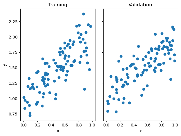

from linear import LinearRegression

LR = LinearRegression()
LR.fit_analytic(X_train, y_train) # I used the analytical formula as my default fit method

print(f"Training score = {LR.score(X_train, y_train).round(4)}")
print(f"Validation score = {LR.score(X_val, y_val).round(4)}")

Training score = 0.6311
Validation score = 0.6072

LR.w.reshape(-1,1)

array([[1.05653571],
       [0.96877292]])

LR2 = LinearRegression()
y2 = y_train.reshape(-1,1)
LR2.fit_gradient(X_train, y2, alpha=0.01)
LR2.w

array([[1.10993122],
       [0.94029021]])

So the weights in both cases are very similar, which means that the gradient method is behaving as it should.

The score also increases monotonically in each iteration.

plt.plot(LR2.score_history)
labels = plt.gca().set(xlabel = "Iteration", ylabel = "Score")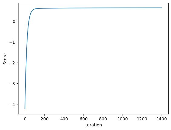

Experiments

Now that we have established that our LinearRegression module is behaving okay, we can move on to experiments, where we increase the number of features and observe the change in validation scores.

n_train = 100
n_val = 100
p_features = np.arange(1,100)
noise = 0.2
train_score = []
test_score = []

# create some data
for i in range(len(p_features)):
    X_train, y_train, X_val, y_val = LR_data(n_train, n_val, p_features[i], noise)
    LR = LinearRegression()
    LR.fit_analytic(X_train, y_train)
    train_score.append(LR.score(X_train, y_train).round(4))
    test_score.append(LR.score(X_val, y_val).round(4))

plt.plot(p_features, train_score, label = 'Training score')
plt.plot(p_features, test_score, label = 'Validation score')
plt.legend()
plt.xlabel('Number of features')
plt.ylabel('Score')
plt.grid()
plt.show()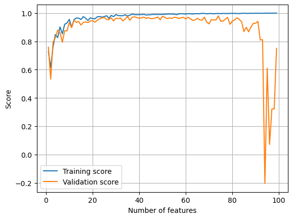

As the number of features increases, the training score approaches 100% while validation score becomes noisier. This demonstrates the effect of overfitting: because the machine is trained to account for every little detail of the training dataset, it becomes too inflexible to work with unseen data.

LASSO Regularization

from sklearn.linear_model import Lasso
L = Lasso(alpha = 0.001)

n_train = 100
n_val = 100
p_features = np.arange(1,100)
noise = 0.2
train_score = []
test_score = []

# create some data
for i in range(len(p_features)):
    X_train, y_train, X_val, y_val = LR_data(n_train, n_val, p_features[i], noise)
    L = Lasso(alpha = 0.001)
    L.fit(X_train, y_train)
    train_score.append(L.score(X_train, y_train).round(4))
    test_score.append(L.score(X_val, y_val).round(4))

plt.plot(p_features, train_score, label = 'Training score')
plt.plot(p_features, test_score, label = 'Validation score')
plt.legend()
plt.xlabel('Number of features')
plt.ylabel('Score')
plt.grid()
plt.show()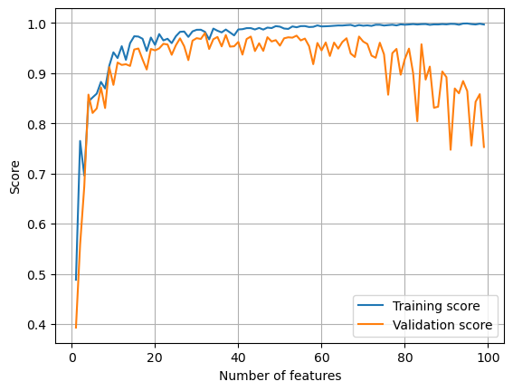

It seems that even when the number of features used is large, the validation score isn’t affected as badly as in the case of pure linear regression. Now we change the strength of regularization to see what changes.

train_score = []
test_score = []

# create some data
for i in range(len(p_features)):
    X_train, y_train, X_val, y_val = LR_data(n_train, n_val, p_features[i], noise)
    L = Lasso(alpha = 0.01)
    L.fit(X_train, y_train)
    train_score.append(L.score(X_train, y_train).round(4))
    test_score.append(L.score(X_val, y_val).round(4))

plt.plot(p_features, train_score, label = 'Training score')
plt.plot(p_features, test_score, label = 'Validation score')
plt.legend()
plt.xlabel('Number of features')
plt.ylabel('Score')
plt.grid()
plt.show()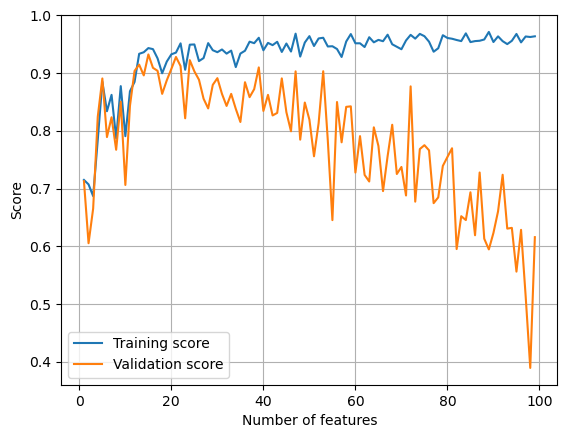

train_score = []
test_score = []

# create some data
for i in range(len(p_features)):
    X_train, y_train, X_val, y_val = LR_data(n_train, n_val, p_features[i], noise)
    L = Lasso(alpha = 0.0005)
    L.fit(X_train, y_train)
    train_score.append(L.score(X_train, y_train).round(4))
    test_score.append(L.score(X_val, y_val).round(4))

plt.plot(p_features, train_score, label = 'Training score')
plt.plot(p_features, test_score, label = 'Validation score')
plt.legend()
plt.xlabel('Number of features')
plt.ylabel('Score')
plt.grid()
plt.show()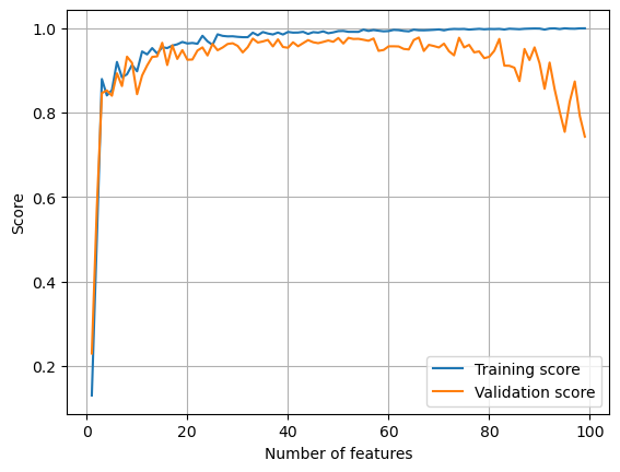

It seems that when the strength of regularization is low, overfitting is less bad.