In this blog post, I will create a machine learning model that predicts an individual characteristic like employment status or income on the basis of other demographic characteristics.
Author
Trong Le
Published
March 25, 2023
In this blog post, I will use the DecisionTreeClassifier module to analyze racial bias in the PUMS dataset of Texas in 2018.
from folktables import ACSDataSource, ACSEmployment, BasicProblem, adult_filterimport numpy as npSTATE ="TX"data_source = ACSDataSource(survey_year='2018', horizon='1-Year', survey='person')acs_data = data_source.get_data(states=[STATE], download=True)acs_data.head()
print('1. There are '+str(len(df)) +' individuals in this survey.')print('2. Of those individuals, '+str(len(df[df['label'] ==1])) +' are employed.')
1. There are 214480 individuals in this survey.
2. Of those individuals, 96805 are employed.
print('3. The number of individuals in each racial group is: \n'+str(df.groupby('group')['label'].aggregate(len)))
3. The number of individuals in each racial group is:
group
1    165969
2     20614
3       836
4        14
5       401
6     10141
7       158
8     10544
9      5803
Name: label, dtype: int64
print('4. The proportion of employed individuals in each racial group is: \n'+str(df[df['label'] ==1].groupby('group')['label'].aggregate(len)/df.groupby('group')['label'].aggregate(len)))
4. The proportion of employed individuals in each racial group is:
group
1    0.455242
2    0.416756
3    0.431818
4    0.357143
5    0.461347
6    0.499359
7    0.430380
8    0.466711
9    0.353955
Name: label, dtype: float64
print('5.1. The proportion of employed male individuals in each racial group is: \n'+str(df[df['SEX'] ==1][df['label'] ==1].groupby('group')['label'].aggregate(len)/df[df['SEX'] ==1].groupby('group')['label'].aggregate(len)))
5.1. The proportion of employed male individuals in each racial group is:
group
1    0.502327
2    0.396673
3    0.474178
4    0.250000
5    0.488263
6    0.553741
7    0.428571
8    0.529160
9    0.371400
Name: label, dtype: float64
C:\Users\ledtr\AppData\Local\Temp\ipykernel_5008\3156142459.py:1: UserWarning: Boolean Series key will be reindexed to match DataFrame index.
  print('5.1. The proportion of employed male individuals in each racial group is: \n' + str(df[df['SEX'] == 1][df['label'] == 1].groupby('group')['label'].aggregate(len)/df[df['SEX'] == 1].groupby('group')['label'].aggregate(len)))
print('5.2. The proportion of employed female individuals in each racial group is: \n'+str(df[df['SEX'] ==2][df['label'] ==1].groupby('group')['label'].aggregate(len)/df[df['SEX'] ==2].groupby('group')['label'].aggregate(len)))
5.2. The proportion of employed female individuals in each racial group is:
group
1    0.410106
2    0.435596
3    0.387805
4    0.500000
5    0.430851
6    0.447318
7    0.432836
8    0.401550
9    0.335905
Name: label, dtype: float64
C:\Users\ledtr\AppData\Local\Temp\ipykernel_5008\266627361.py:1: UserWarning: Boolean Series key will be reindexed to match DataFrame index.
  print('5.2. The proportion of employed female individuals in each racial group is: \n' + str(df[df['SEX'] == 2][df['label'] == 1].groupby('group')['label'].aggregate(len)/df[df['SEX'] == 2].groupby('group')['label'].aggregate(len)))
Except for groups 2, 4 and 7, the other racial groups have a higher proportion of employed men than women.
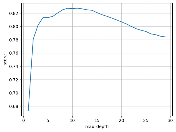
Now we will train our model. I’m using the DecisionTreeClassifier model. Below is my code to see which maximum depth of the tree gives the most accuracy. The cross-validation is only done on the training data.
It seems that max_depth = 9 is our optimal tree depth. We will now test this model on test data.
model = make_pipeline(StandardScaler(), DecisionTreeClassifier(max_depth =9))model.fit(X_train, y_train)y_hat = model.predict(X_test)score = (y_hat == y_test).mean()print('1. The overall accuracy of the model is '+str(score.round(4)) +'.')from sklearn.metrics import confusion_matrixC = confusion_matrix(y_test, y_hat, normalize='true')TN = C[0][0]FP = C[0][1]FN = C[1][0]TP = C[1][1]PPV = TP/(TP+FP)print('2. The overall positive predictive value is '+str(PPV.round(4)) +'.')print('3. The overall false negative rate is '+str(FN.round(4)) +' and false positive rate is '+str(FP.round(4)) +'.')
1. The overall accuracy of the model is 0.8237.
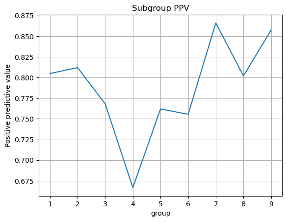
2. The overall positive predictive value is 0.8045.
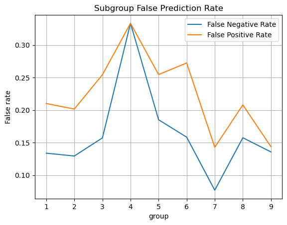
3. The overall false negative rate is 0.1361 and false positive rate is 0.2099.
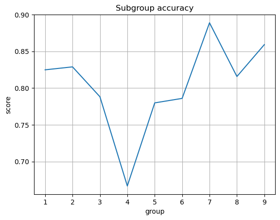
This model is approximately calibrated. If we exclude group 4, which has a small sample size of 14 individuals, the positive predictive value for each group is close to the overall PPV. It is the same case for the FNR and FPR, which means that this model also satisfies approximate error rate balance. This means that our model has the same prevalence for all groups, which means that this is an amazing model!
Conclusion
This model can be used by job referrals websites such as LinkedIn to advertise to potentially unemployed people. It can also be used by car insurance companies to advertise to potentially employed people, who may own a car to commute to work. Or it can be used by apartment complexes to advertise to employed people.
I think that if this model is used in a governmental setting, the model can predict the employability of a person based on their features excluding race. This can be used to decide whether a person is eligible for a loan (if they can pay back the loan by working at a job), whether they can rent a place in a certain area (expensive areas require a stable and supple income).
Based on my audit, my model does not have any problematic bias.
A problem with my model is that it cannot accurately predict for racial groups that have too few individuals.